Pressure Loss in Fluid Flow

Pressure Loss in Fluid Flow

A comprehensive analysis of energy loss in fluid systems, with practical applications for hydraulic engineering and the hydraulic fluid tractor industry.

Fluid flow visualization showing pressure differentials in a pipe system

Introduction to Pressure Loss

Real fluids possess viscosity, which creates resistance when they flow. To overcome this resistance, flowing liquids must expend a portion of their energy. This energy loss is represented by the hg term in the Bernoulli equation for real fluids, as shown in equation (2-23). When converted to pressure loss, this can be expressed as Δp = ρghg.

In hydraulic systems, including the hydraulic fluid tractor, pressure loss converts hydraulic energy into heat, which can cause increased system temperature. Therefore, when designing hydraulic systems—whether for industrial machinery or a hydraulic fluid tractor—it is crucial to minimize pressure loss.

Pressure losses can be categorized into two main types: frictional pressure losses along pipelines and local pressure losses. Each type has distinct characteristics and calculation methods, which we will explore in detail. Understanding these losses is particularly important for optimizing the performance of a hydraulic fluid tractor, where efficiency directly impacts productivity and operating costs.

Diagram showing pressure loss in different sections of a hydraulic system
Figure 1: Pressure distribution in a typical hydraulic circuit, demonstrating energy loss through the system

I. Frictional Pressure Losses

Frictional pressure loss refers to the pressure loss caused by viscous friction when fluid flows through straight pipes of constant diameter. The magnitude of this loss varies depending on the flow regime. In applications like the hydraulic fluid tractor, where efficient fluid transmission is critical, accurately calculating these losses ensures optimal system design.

A. Laminar Flow Frictional Losses

In laminar flow, fluid particles move in an orderly manner, allowing us to use mathematical methods to fully explore their flow conditions and derive formulas for calculating frictional pressure losses. This is particularly relevant for components of a hydraulic fluid tractor operating at lower speeds where laminar flow conditions prevail.

Velocity profile of laminar flow in a pipe showing parabolic distribution
Figure 2: Laminar flow velocity profile in a straight pipe, illustrating the parabolic distribution

1. Velocity Distribution in Flow Cross-Section

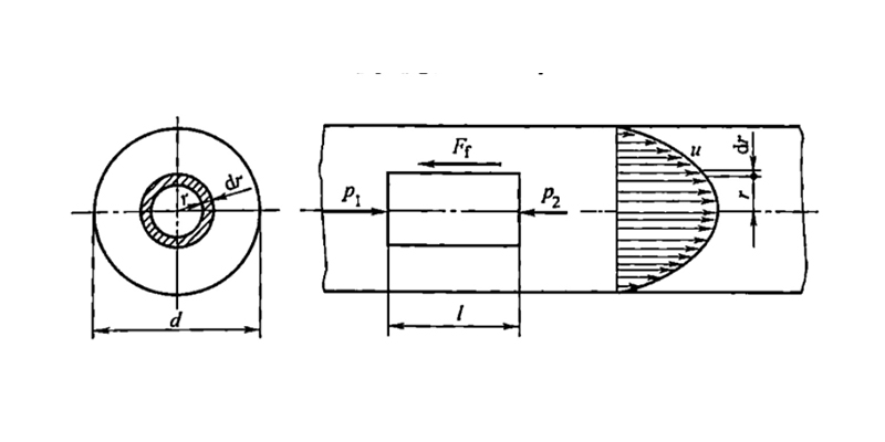
Consider the laminar flow of a hydraulic fluid tractor's operating fluid in a horizontal straight pipe of constant diameter, as shown in Figure 2-14. A small cylindrical element coinciding with the pipe axis is taken as the study object. Let its radius be r, length be l, the pressures acting on its two end faces be p₁ and p₂, and the internal friction force acting on its side surface be Ff.

When the fluid flows at a constant velocity, it is in a state of force equilibrium, so:

(p₁ - p₂)πr² = Ff

According to Newton's law of viscosity, Ff = -2πrlμ(du/dr) (the negative sign indicates that velocity u decreases as r increases). Letting Δp = p₁ - p₂ and substituting Ff into the above equation, we get:

Δp·πr² = -2πrlμ(du/dr)

Rearranging gives:

du = - (Δp / (2μl)) r dr

Integrating this equation and applying the boundary condition that u = 0 when r = R (where R is the pipe radius), we obtain:

u = (Δp / (4μl))(R² - r²) (2-27)

This shows that the velocity of liquid particles in the pipe follows a parabolic distribution in the radial direction. The minimum velocity occurs at the pipe wall (r = R) where umin = 0, while the maximum velocity is at the pipe axis (r = 0) where umax = (Δp R²)/(4μl) = (Δp d²)/(16μl) (where d is the pipe diameter).

2. Flow Rate Through the Pipe

For a small annular flow cross-section with radius r and width dr, its area is dA = 2πrdr, and the flow rate through it is:

dQ = u dA = 2πru dr = 2πr·(Δp / (4μl))(R² - r²) dr

Integrating this from r = 0 to r = R gives:

Q = ∫₀ᴿ (πΔp / (2μl))(R²r - r³) dr = (πΔp R⁴) / (8μl) = (πΔp d⁴) / (128μl) (2-28)

3. Average Velocity in the Pipe

According to the definition of average velocity v, we have:

v = Q / A = (πΔp d⁴ / 128μl) / (πd² / 4) = (Δp d²) / (32μl) (2-29)

Comparing equation (2-29) with the maximum velocity umax, we find that the average velocity v is half of the maximum velocity umax.

4. Frictional Pressure Loss

Rearranging equation (2-29) gives the frictional pressure loss:

Δpλ = (32μlv) / d²

This shows that for laminar flow in straight pipes, the frictional pressure loss is proportional to the pipe length, flow velocity, and dynamic viscosity, and inversely proportional to the square of the pipe diameter. This relationship is crucial for designing efficient fluid transport systems, including those in a hydraulic fluid tractor.

Rewriting the equation in a more convenient form for practical calculations:

Δpλ = λ (l/d) (ρv²/2) (2-30)

where λ is the friction coefficient. For laminar flow in circular pipes, the theoretical value is λ = 64/Re. However, considering possible deformation of the actual circular pipe cross-section and potential cooling of the liquid layer near the pipe wall, in practical calculations, λ = 75/Re for metal pipes and λ = 80/Re for rubber hoses commonly used in hydraulic fluid tractor systems.

Equation (2-30) was derived for horizontal pipes. Since the pressure changes caused by the self-weight of the liquid and positional changes are small and can be neglected, this formula also applies to non-horizontal pipes, such as those found in various orientations within a hydraulic fluid tractor.

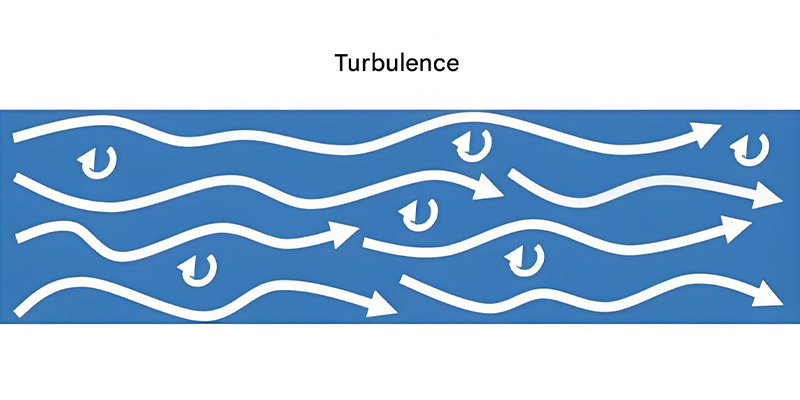
B. Turbulent Flow Frictional Losses

The formula for calculating frictional pressure loss in turbulent flow has the same form as in laminar flow, i.e., Δpλ = λ (l/d) (ρv²/2). However, the friction coefficient λ in this case depends not only on the Reynolds number Re but also on the pipe wall roughness, expressed as λ = f(Re, Δ/d), where Δ is the absolute roughness of the pipe wall and Δ/d is the relative roughness.

Turbulent flow visualization showing chaotic fluid movement
Figure 3: Turbulent flow characteristics showing irregular fluid motion and eddy formation

For smooth pipes, λ = 0.3164Re-0.25. For rough pipes, the value of λ can be found from relevant charts in engineering handbooks based on different Re and Δ/d values. These charts are essential references for designing efficient hydraulic systems, including components of a hydraulic fluid tractor operating under turbulent conditions.

The absolute roughness of pipe walls varies with the pipe material. For general calculations, the following values can be referenced:

  • Steel pipes: 0.04 mm
  • Copper pipes: 0.0015~0.01 mm
  • Aluminum pipes: 0.0015~0.06 mm
  • Rubber hoses (common in hydraulic fluid tractor systems): 0.03 mm

Practical Note for Hydraulic Systems

In hydraulic fluid tractor design, selecting appropriate pipe materials and diameters based on expected flow conditions is critical. Turbulent flow generally creates higher pressure losses, so system designers often aim to maintain laminar or transitional flow regimes in critical components to improve efficiency and reduce operating costs.

II. Local Pressure Losses

Local pressure loss occurs when fluid flows through pipe elbows, fittings, sudden changes in cross-section, valve ports, filters, and other local devices. In these regions, the flow creates eddies and exhibits intense turbulence, resulting in significant energy loss. These components are numerous in a hydraulic fluid tractor, making local losses a major consideration in system design.

When fluid flows through these various local devices, the flow conditions are extremely complex with many influencing factors. Theoretical analysis and calculation of local pressure loss values are therefore difficult. Instead, the local resistance coefficient ζ is generally determined experimentally. The formula for calculating local pressure loss is:

Δpζ = ζ (ρv² / 2) (2-31)

where ζ is the local resistance coefficient. Values of ζ for various local device structures can be found in relevant engineering handbooks, which are essential references for hydraulic fluid tractor designers.

The local pressure loss when fluid flows through various types of valves can also be calculated using equation (2-31). However, due to the complex internal channel structures of valves—common components in any hydraulic fluid tractor—calculation using this formula is relatively difficult. Therefore, the practical calculation formula for the local pressure loss Δpv of valve components is:

Δpv = Δpn (q / qn)² (2-32)

where qn is the rated flow rate of the valve, Δpn is the pressure loss of the valve at the rated flow rate qn (which can be found in the valve's product specifications or design handbooks), and q is the actual flow rate through the valve. This formula is particularly useful when selecting valves for a hydraulic fluid tractor, ensuring that pressure losses remain within acceptable limits.

Common Local Resistance Coefficients (ζ)

  • Sudden expansion (large/small = 5): 1.0
  • Sudden contraction (small/large = 0.5): 0.4
  • 90° elbow (standard): 1.5
  • 45° elbow (standard): 0.3
  • Globe valve (fully open): 10~15
  • Ball valve (fully open): 0.5~1.0

Pressure Loss Considerations

In hydraulic fluid tractor design, local losses typically account for 30-50% of total system pressure loss.

Proper component layout can reduce local losses by 20-30%.

Using gradual transitions instead of sudden changes can reduce ζ values by 50-70%.

III. Total Pressure Loss in Pipe Systems

The total pressure loss in an entire pipe system is the sum of all frictional pressure losses and all local pressure losses, expressed as:

ΣΔp = ΣΔpλ + ΣΔpζ + ΣΔpv = Σ[λ(l/d)(ρv²/2)] + Σ[ζ(ρv²/2)] + ΣΔpv (2-33)

In hydraulic systems, including the hydraulic fluid tractor, most pressure losses are converted into heat, causing increased system temperature and potential leakage, which can affect system performance. From the pressure loss calculation formulas, it is evident that reducing flow velocity, shortening pipe lengths, minimizing sudden changes in pipe cross-sections, and improving the machining quality of pipe inner walls can all reduce pressure losses.

Among these factors, flow velocity has the most significant impact. Therefore, the flow velocity of liquids in pipe systems should not be too high. However, excessively low velocities will increase the size and cost of pipes and valve components. For a hydraulic fluid tractor, finding the optimal balance between velocity, component size, and system cost is crucial for achieving both performance and economic efficiency.

Figure 5: Comparison of pressure loss components in a typical hydraulic fluid tractor system

Design Optimization Strategies

To minimize pressure losses in hydraulic systems like the hydraulic fluid tractor:

  1. Select appropriate pipe diameters to maintain optimal flow velocities (typically 1-5 m/s for hydraulic systems)
  2. Minimize total pipe length through careful system layout
  3. Use gradual bends and transitions instead of sharp elbows
  4. Choose valves and fittings with low resistance coefficients
  5. Group components to reduce connection piping
  6. Regularly maintain filters to prevent clogging, which significantly increases local losses

Example Calculation

In the hydraulic system shown in Figure 2-15, which resembles the hydraulic circuit of a small hydraulic fluid tractor, the following parameters are known: pump flow rate q = 1.5×10⁻³ m³/s, hydraulic cylinder inner diameter D = 100 mm, load F = 30000 N, return chamber pressure is approximately zero. The supply pipe to the hydraulic cylinder is a steel pipe with inner diameter d = 20 mm, total length equal to the vertical height H = 5 m. The total local resistance coefficient for the supply line ζ = 7.2. The hydraulic oil density ρ = 900 kg/m³, and the kinematic viscosity at operating temperature ν = 46 mm²/s.

Hydraulic system diagram for pressure loss calculation example
Figure 6: Schematic diagram of the hydraulic system used in the calculation example

Calculate:

  1. Pressure loss in the supply line
  2. Pump supply pressure

Solution:

(1) Calculating pressure loss in the supply line

Flow velocity in the supply pipe:

v = q/A = (1.5×10⁻³) / [(π/4)×(20×10-3)²] = 4.77 m/s

Reynolds number:

Re = (vd)/ν = (4.77×20×10-3) / (46×10-6) = 2074 < 2320 (laminar flow)

Friction coefficient (for steel pipes):

λ = 75/Re = 75/2074 = 0.036

Therefore, the pressure loss in the supply line is:

ΣΔp = [λ(l/d) + Σζ] × (ρv²/2) = [0.036×(5/0.02) + 7.2] × (900×4.77²/2) Pa = 0.166×10⁶ Pa = 0.166 MPa

(2) Calculating pump supply pressure

Applying the Bernoulli equation between the pump outlet pipe section 1-1 and the section 2-2 after the hydraulic cylinder inlet:

p₁ + ρgh₁ + (α₁ρv₁²)/2 = p₂ + ρgh₂ + (α₂ρv₂²)/2 + ΣΔpw

Expressing this in terms of p₁:

p₁ = p₂ + ρg(h₂ - h₁) + (ρ/2)(α₂v₂² - α₁v₁²) + ΣΔpw

Where:

p₂ is the working pressure of the hydraulic cylinder:

p₂ = F/A = 30000 / [(π/4)×(100×10-3)²] = 3.81×10⁶ Pa = 3.81 MPa

ρg(h₂ - h₁) is the potential energy change per unit volume of liquid:

ρg(h₂ - h₁) = ρgH = 900×9.8×5 Pa = 0.044×10⁶ Pa = 0.044 MPa

(ρ/2)(α₂v₂² - α₁v₁²) is the kinetic energy change per unit volume of liquid. For laminar flow, α = 2.

The velocity in the hydraulic cylinder:

v₂ = q/A = (1.5×10⁻³) / [(π/4)×(100×10-3)²] = 0.19 m/s

Thus:

(ρ/2)(α₂v₂² - α₁v₁²) = (900/2)×(2×0.19² - 2×4.77²) Pa = -0.02×10⁶ Pa = -0.02 MPa

ΣΔpw is the total pressure loss in the supply line:

ΣΔpw = 0.166 MPa

Therefore:

p₁ = (3.81 + 0.044 - 0.02 + 0.166) MPa = 4 MPa

From the calculation of p₁ in this example, we can see that in hydraulic transmission systems like the hydraulic fluid tractor, the pressure changes caused by liquid position height variations and flow velocity changes are relatively small. In general calculations, the terms ρg(h₂ - h₁) and (ρ/2)(α₂v₂² - α₁v₁²) can be neglected. Therefore, the expression for p₁ can be simplified to:

p₁ = p₂ + ΣΔp (2-34)

Although equation (2-34) is an approximate formula, it is widely used in hydraulic system design calculations, including the design and analysis of hydraulic fluid tractor systems.

Practical Application in Hydraulic Fluid Tractor Design

This example demonstrates the typical pressure loss calculations required when designing a hydraulic fluid tractor. The 4 MPa pump pressure calculated includes both the working pressure needed to overcome the load and the necessary pressure to compensate for system losses. In actual hydraulic fluid tractor design, these calculations would be repeated for all critical circuits, including lifting, steering, and implement systems, to ensure efficient operation and component sizing.

Understanding pressure loss in fluid systems is fundamental to designing efficient hydraulic systems, from industrial machinery to agricultural equipment like the hydraulic fluid tractor. Proper calculation and minimization of both frictional and local losses ensure optimal performance, reduced energy consumption, and extended component life.

Learn more
滚动至顶部